B. Technical
Explanation of the Data
WHY A DATA HYPERCUBE ?
The DSDP led to many revolutionary advances in our
understanding of earth and ocean history over 200 million years. Much
of the observational data that underpinned the science is
contained in this project. The project has reformed the data to
allow
bulk analysis and visualisation of trends in global-scale earth
history, as seen through lithologies.
This was best achieved by forming a
multidimensional data structure - a hypercube. Until now re-processing,
large scale computer
visualization and
analysis of the data was not possible. It was held pagewise as a type
of written-corelog, unsuitable for
spreadsheets,
geographic information systems and databases. To make the dataset
available for use in such applications it has had to be brought into a
cellular format, and descriptive data has had to be parsed
linguistically. The other major issues are data sparsity (the sheer
amount of null values across the samples*parameters matrix), database
granularity, and data quality control.
By describing the data as a 'hypercube' we want to convey
that the whole of these geological data data can now be cut, viewed and
analysed in many different
planes, by the XYZT coordinates (longitude, latitude, depth bSL, depth
bSF, geologic time) and also by one parameter against another. If
people think of a multi-dimensional cube of information, admittedly
with many gaps, then they will be correct.
Of course, a poly-dimensional data hypercube (this one is 4
dimensional at minumum, XYZT) cannot truly be imagined. Likewise, data
products from that concept of the data have to live in the
reality of various common software applications. Hypercubes are
rendered to humans by operations such as projecting to planes or
volumes, and 'splatting' (e.g., Yang 2003). We happen to render the
data in ways
that are strongly spatially directed, but inter-parameter splats are
equally possible with the set.
In the NGDC CDROM, the best organized collection of
DSDP
data, the database granularity remained at drillsite "hole" level,
unless items were extracted manually from the page-long hole
descriptions. With this project, the data per core section is
broken out into separate data items, a granularity of approximately
1.5m vertically. However, in many instances we have been able to
discern and treat observations on individual small segregations and
fractions within the
core sections, giving a granularity on the scale of centimetres.
The data sparsity of this project is considerable. Only
about 23% of the [parameter*sample] matrix holds non-null values. This
is
partly because not all observations are made on all samples in the
on-board or lab programs. However it is also due to that fact that not
all the lithologic descriptions could be parsed successfully,
especially where the
prose was irregular. Some of the analytical results will also have
failed at quality filters.
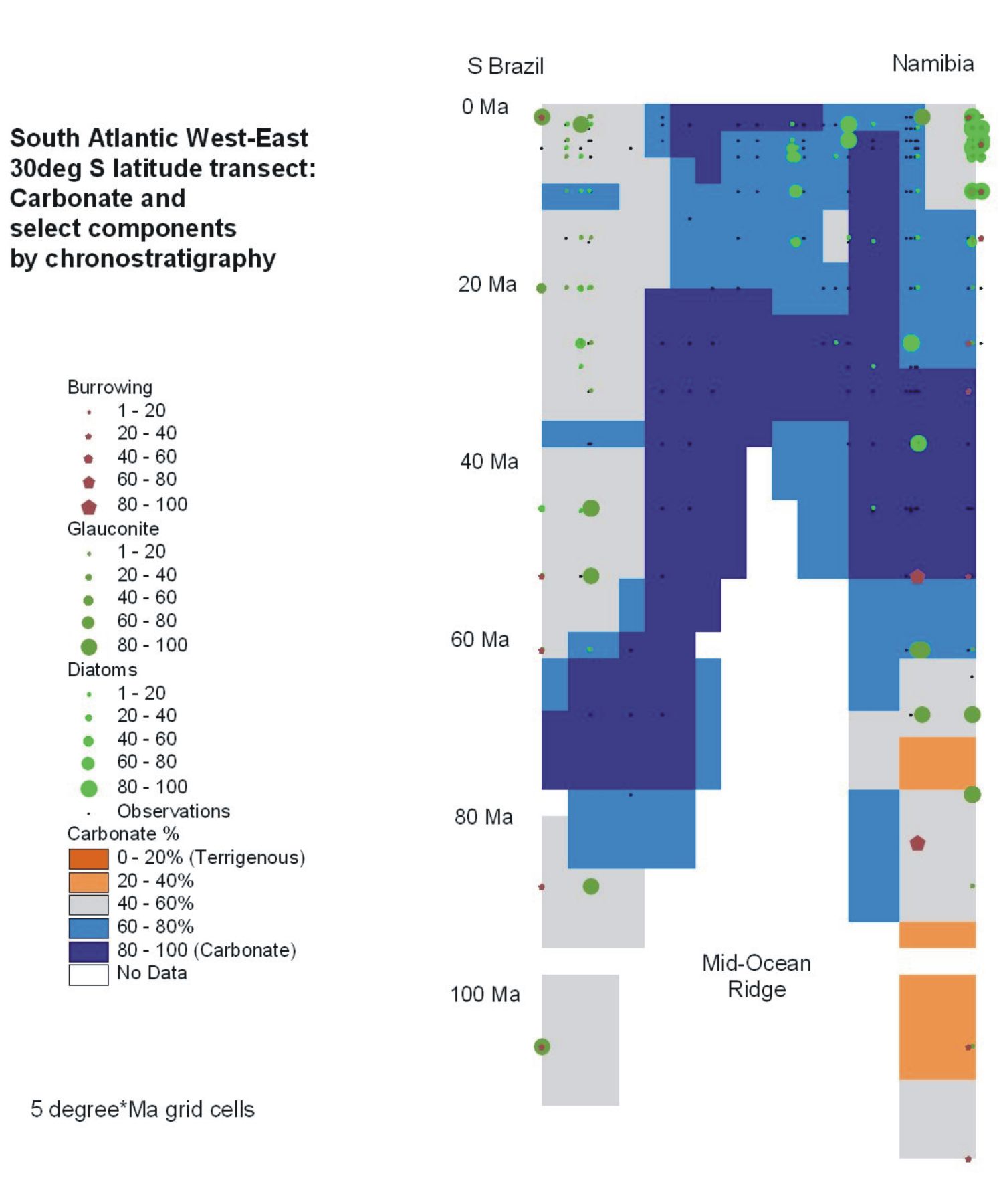
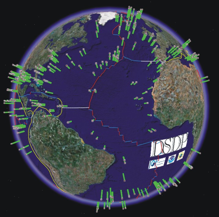
The illustration along-side this introduction and others at
THIS_PAGE show what is possible now, using the hypercube. Basically,
with this in place, it is possible to voxelize aspects of ocean
lithologic history, akin to the gridding on flat maps.
|
Time
Coordinate
Geological time in the original DSDP data was given in
terms of
period, stage, and zone biostratigraphic and chronostratigraphic terms.
Only rarely were absolute isotopic or paleomagnetic ages attached to
materials. Unfortunately, but inevitably, the geologic time scales in
use evolved during DSDP, and on-board
age determinations were interim. Lazarus et al. (1995) developed age-depth
models for 88 of the drilled holes according to one time scale and
those models are refined, extended and served now through Chronos (2007). The revisions of time
scales and time terms were not propagated systematically through the
DSDP data, though some post-cruise datings were merged in during
creation of the CDROM compilation.
We have taken the CDROM age determinations such as "Early
Oligocene" and applied the International Stratigraphic Commission (ICS)
timescale (Gradstein et al. 2004)
to those names. This is
a simplistic approach, admittedly, but we look to qualified
geochronologists to replace these ages with better calibrated
values in the future. The assessed scale of error in the method is of
the order of <1My (exceptionally up to 4My) to judge from
successive revisions of stage absolute ages (Gradstein et al. 2004).
The method of parsing the age terms was as follows. Age
values are encountered in the CDROM 'AGEPROF' or 'PALEO' lines, given
usually as a stage name, perhaps with a division like "early". In the
dbSEABED dictionary
the chronological unit names are assigned absolute values (e.g. entry,
"rupeln,Rupelian
Stage,date,28.4,33.9,0.1, 0.1") of youngest, oldest, youngest
uncertainty, oldest uncertainty. The unit is millions of years (my).
The parser uses the youngest/oldest limits to create a code like
"28.4y:o33.9" (with the uncertainties e.g., "28.4[0.1]y:o33.9[0.1]").
An analysed age such as K-Ar dating
will appear in EXT (e.g., "0.0023[0.0001]y:o"), a
biostratigraphic age in PRS. Where an age range
is given, such as "upper_oligocene to lower_miocene" the two
age ranges are combined, giving in this case the result "15.97t:b28.4".
So that data can be plotted to GIS, the code is transferred
to a single
central value in the preparation of the DSD_***n and Shapefile
filesets. So that all samples have a time coordinate, just as they have
a geographic coordinate, an age-depth index was built and was used to
spread the age values throughout entire the DSD_***n and Shapefile
filesets. Undated samples took the age of the sample next above.
|
Vertical
Coordinate
- The vertical datums used during data collection and
archiving have been an impediment to creating a global analysable
structure from ocean lithologic data. In this project we retain the
original values, but the prime vertical coordinate is altitude relative
to present sealevel. By using altitudes we keep the proper handedness
of the data. Of course, sealevel is an inexact datum, but the
variations are unlikely to be an issue except for closed-spaced or
re-occupied DSDP holes.
- We attach a sequential number - Sample Key - to each
observed unit, segregation, sample, phase or fraction: in short to each
different analysed material. Some samples are subject to many different
analyses, and then one key applies to all those analyses. High value is
obtained from this because it allows inter-parameter comparisons. When
an observation is made at different scales, such as a visual
description versus a smear slide, that counts as different material and
key.
- A code for the DSDP Leg, Site, Hole, Core and Section is
given for each material (e.g., "DSDP:23:310:A:15:6") and can be used in
relational databases. Other details on the sectioning and labelling of
the core materials is provided by NOAA (2000).
|
Process
Trail
A feature of dbSEABED outputs is the "DataType" or Audit
Code. In first-level outputs it holds record of the data themes that
contribute to an output record, for instance "LTH.COL.GTC" for
lithology, colour, geotechnical. It will be different for extracted and
parsed outputs. On merging these, as is done for the ONE and WWD output
levels, DataType records whether a parameter is extracted (i.e.,
analysed, numeric) or parsed (i.e., descriptive, word-based), or
specially calculated (estimated). A sequence
like"PPPxPPxxxxPEEEPExxxPE" shows the EXT, PRS, CLC origins of the next
20 parameters, from 'Gravel' to 'GeolAge'.
|
File formats
representing the
hypercube
- From this web site, three types of data products can be
obtained, expressions of the hypercube:
- Text files in GIS format presenting the data ready for
use on geographic, chronologic, or inter-parameter coordinates
- ArcMAP / ArcSCENE shapefiles, both geographic XYZ and
geologic time XYT coordinates
- A Google Earth top-level indexing of the data
- File naming is as follows: DSD - Deep-Sea Drilling Project
processing project; XXX - data processing stream (e.g., 'EXT'); * -
either N for NGDC data delivery format, or C for compressed components
format. The result is "DSD_XXX*", usually text. Shapefiles generated by
ArcCatalog have "XY#" to the front, where # is the type of vertical
dimension, Z for depth, T for geologic time.
- The null default values are "-99" for integer, "-99.0" for float, and "-" for string. They signify "No Data".
|
Text
file collection
- The primary text files are in DSD_TEXT_Files.zip.
There is no folder
structure involved, so they can be extracted to any location.
- DSD_EXTn - Extracted data,
taken
from inputs with little processing necessary. Mainly from analytical
results in numerical and coded formats.
- DSD_PRSn - Parsed results,
based
on the descriptive word-based data.
- DSD_CLCn - Results from
further
calculations following the extracted / parsed results. Mainly for
abstruse parameters, chiefly geoacoustic, geotechnical.
- DSD_ONEn - merged results of
the
EXT, PRS, CLC processing streams. The merging is done by priority that
favours PRS over EXT over CLC, where more than one is present. Except
for grainsizes, the process operates per parameter. For grainsizes, the
most complete suite of grainsize data (gvl, snd, mud, grsz, srtng) is
taken from the PRS,EXT,CLC data, prioritized where two or more equal
suites are present.
- DSD_CMPn - Component and
feature
abundances and intensities, computed from inputs such as grain counts,
visual descriptions, etc. Component abundances sum to at most 100%,
feature intensities (suffix "_F") are each limited to 100%.
|
Outputs
specially formatted
- These are also in the zip file DSD_TEXT_Files.zip:
- dsd_CMPc - condensed
components/features data for use in
servers like GeoMapApp which draw on the data using a script.
- dsd_AGES - special listing of age
identifications in a format compatible with the accompanying
reformatted Lazarus et al. (1995)
listing.
|
GIS
FORMATTED OUTPUTS
(ArcMap, ArcView, ArcScene)
Shapefiles
- The text files above can be plotted, queried, sub-setted,
symbolized, gridded in GIS systems including those of the ESRI suite.
Shapefiles for the DSD_PRSN and DSD_CMPn series have been prepared and
are served here. Only in ArcScene will the 3-dimensional aspect of the
files be visible. Notice that for correct handedness in GIS, depths
below sealevel and geologic time are negative (altitudes,
time's arrow).
- A global baseline to start with is the
low-resolution public ESRI country.shp
layer of national outlines.
Users will later be able to make
gridded or mesh topographies (bathymetries) to 'hang' the DSDP cores
below.
- The Shapefile sets are either in physical depth XYZ or
geologic time XYT coordinate systems, using WGS84 datums. They follow
the file types listed above for the text files. They are
downloadable in zipped form from XYZ_Coordinates
and XYT_Coordinates
(337Mb each unzipped). ArcView 3.x GIS also opens these shapefiles.
- Legends suitable for the data can be obtained from the
dbSEABED site
"http://instaar.colorado.edu/~jenkinsc/dbseabed/legends/". There is a
collection for ArcView 3.x ('Avls') and for ArcMap9.x/ArcScene
('Lyrs'), point legends only.
|
|
Explanatory
Documentation
- Detailed documentation of dbSEABED methods, standards and
outputs can be found on the web, especially under the usSEABED
EEZ-mapping project. Good point-of-entry URL's are the Processing
methods and FAQ web pages of Jenkins (2005a,b).
- A document describing details of the processing of the DSDP
data is
available at NOAA (2000b).
|
Version
notes
- This is delivery v1.1 to MGG NGDC in Boulder. (v1.0 was
initial
assessment). The format of files may change if required by methods of
serving / display.
- Some aspects of the data that could do with
further development.
- The main one is that
the geochronology is based on (?)shipboard paleontology. This should be
replaced
by the Lazarus scheme (NGDC dataset) at least, but also preferably with
a new
compilation by LDEO. Since the hypercube integration is computational,
any new
chronologies can be spliced in efficiently.
- Not all the
descriptive data could be
successfully parsed. You can imagine that that is the case with some of
the
prose used by the describing scientists. On my assessment over 70% are
parsed,
and with an improved left-hand parser which is near complete, that will
rise to
over 90%.
- Only 72
of the numerous possible components/features are listed. Future
versions may extend to the complete (but evolving) set that is
available from the data and the dbSEABED dictionary.
- Not all the
parameter themes of the CDROM have been incorporated. The most glaring
absence is GRAPE, but also not treated yet are:
- The subbottom
depths are rendered exactly as given in the DSDP CDROM of input data. A
conversion to later schemes may be possible in the future. Notice that
by convention the way of placing sections in core lengths was changed
at Leg 46.
- The sample
depths are only approximately in depth order, but are in strict order
by section. Some top and bottom depth
values may be reversed, where observers made that error.
|
References
- Chronos, 2007. Chronos.
Iowa State University, Department of Geological and Atmospheric
Sciences
[Online: "http://www.chronos.org/"]
- Gradstein, F.M., Ogg, J.G., and Smith,
A.G., Agterberg, F.P., Bleeker, W., Cooper, R.A., Davydov, V., Gibbard,
P., Hinnov, L.A., House, M.R., Lourens, L., Luterbacher, H.P.,
McArthur, J., Melchin, M.J., Robb, L.J., Shergold, J., Villeneuve, M.,
Wardlaw, B.R., Ali, J., Brinkhuis, H., Hilgen, F.J., Hooker, J.,
Howarth, R.J., Knoll, A.H., Laskar, J., Monechi, S., Plumb, K.A.,
Powell, J., Raffi, I., Röhl, U., Sadler, P., Sanfilippo, A.,
Schmitz,
B., Shackleton, N.J., Shields, G.A., Strauss, H., Van Dam, J., van
Kolfschoten, T., Veizer, J., and Wilson, D., 2004. A Geologic Time Scale 2004.
Cambridge University Press, 589 pages.
- Jenkins, C.J., 2005a. dbSEABED. In: Reid, J.M., Reid, J.A.,
Jenkins, C.J., Hastings, M.E., Williams, S.J. and Poppe, L.J., 2005. usSEABED: Atlantic Coast Offshore Surficial Sediment
Data Release, version 1.0. U.S. Geological Survey Data Series 118.
[Online: "http://pubs.usgs.gov/ds/2005/118/htmldocs/dbseabed.htm"]
- Jenkins, C.J., 2005b.
Frequently Asked Questions (FAQs) about dbSEABED. In: Reid, J.M., Reid,
J.A., Jenkins, C.J., Hastings, M.E., Williams, S.J. and Poppe, L.J.,
2005, usSEABED: Atlantic Coast Offshore
Surficial Sediment Data Release, version
1.0. U.S. Geological Survey Data Series 118.
[Online: "http://pubs.usgs.gov/ds/2005/118/htmldocs/faqs.htm"]
- Lazarus, D., Spencer-Cervato, C., Pika-Biolzi, M.,
Beckmann, J,P., von Salis, K., Hilbrecht, H. and Thierstein, H., 1995.
Revised Chronology of Neogene DSDP Holes from the World Ocean. Ocean Drilling Program Technical Note # 24.
[Online: "http://www.ngdc.noaa.gov/mgg/geology/lazarus.html"]
- NOAA, 2000a. Core
Data from the Deep Sea Drilling Project. WDC
for MGG, Boulder Seafloor Series volume 1. [CDROM; Online:
"http://www.ngdc.noaa.gov/mgg/geology/dsdp/start.htm"]
- NOAA, 2000b. Documentation files for DSDP data.
In: NOAA, 2000a. [CDROM; Online:
"http://www.ngdc.noaa.gov/mgg/geology/dsdp/doc/docs.htm"]
- Ryan, W.B. and Carbotte, S.M. 2009.
GeoMapApp. [URL:
"www.marinegeo.org/geomapapp"]
- Yang, L., 2003. Visual Exploration of Large Relational Data
Sets through 3D Projections and Footprint Splatting. IEEE Trans. Knowl. Data Engng.,
15(6), 1460-1471.
|