|
Introduction
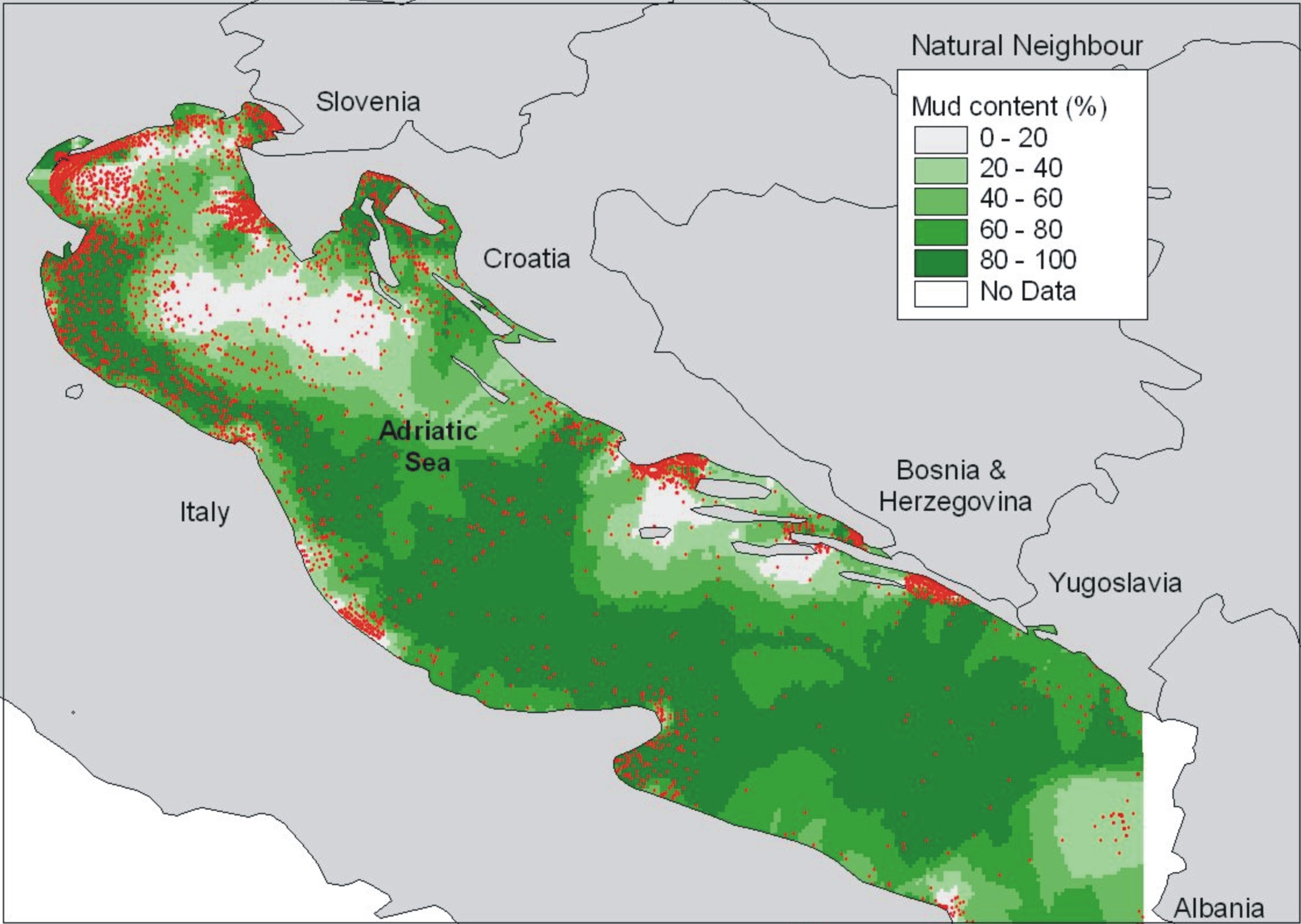
The most useful and visually presentable outputs from dbSEABED are
gridded data, where map cells of size about 1km2 are
assigned a parameter value, for instance on seabed mud content or
average grainsize. Gridded
maps are very suitable as illustrations in papers, for input to
numerical models, and to drape on 3d surfaces.
Unfortunately,
making the grids involves interpolation, a field of spatial data
handling that is difficult and involves judgement. There is a
bewildering choice of interpolation methods and statistical
reliabilities, are very dependent on
choice of
interpolator and quality of the input data distribution. The
reliabilities are usually only 80% at
best (Cressie
1993; Dubois et al., 1998; Bengio et
al.,
2004).
Existing
interpolators
Many GIS have embedded interpolators, including Inverse Distance
Weighting (IDW), Kriging, Polynomial/Spline, Optimal Interpolator, and
Natural Neighbour types. Experience shows that in almost every case
those 'black box' interpolators give spurious results for seabed
mapping, especially in coastal areas. The list of difficulties includes
these:
- Boundaries of offshore sediment
zones are badly formed; they are
often made to cross obvious environmental zonations (such as water
depths) and of course, the coastlines.
- Where inshore data is scarce
(usually the case), properties of
the offshore sediments
are drawn in too close to the coastlines.
- Whenever a wide search radius
is
set to deal with the sparse-data deep-water
zones, good detailed information for well-mapped shallow areas is
smeared.
- Global interpolators -
particularly the spline, polynomial and trend-surface methods - are
particularly bad and make false highs and lows in areas of sparse data.
- Sediment / rock distributions
on the seabed can have sharp
boundaries (e.g., Cacchione et al. 1984; imagery in Intelman et al.,
2007). They are not mapped accurately using Kriging,
Polynomials, or Optimal Interpolation which produce
continuous-differentiable results more suitable for water
properties and potential surfaces like gravity.
- The error (uncertainty) calculated by Kriging and
Optimal
Interpolation are measures of local internal consistency of the
data, not a full error analysis involving measurement error,
assumptions (e.g., semivariogram model; Tomczak 2003), and
other uncertainties.
- Point data selection is distance based only. Strongly
asymmetric
results can result for gridcells lying near data clusters.
In some ways, these shortcomings
represent the fact that most
interpolation packages are unalloyed mathematical methods. In order to
address points above, the mathematical processes need to be modified
(i.e., directed and tuned). By doing this, we introduce factors that a
human
would use to contour data and make a result that fits better with
expert knowledge of an area, for instance its environmental zonations.
Of course, though, the mathematical underlay is necessary for rigour
and to handle the large data volumes.
Competent
Seabed Interpolator (CSI)
To resolve these issues an interpolator has been written for use with
seabed data, in particular with dbSEABED datasets. It is called
"competent": adequate for the job, fit for purpose; but capable of
improvement. It was written to meet a
recurring need for reliable grid generation from dbSEABED. The software
is publicly
released, open for modification, and can
be used for data from
other sources. (Readme.txt)
The advantages of CSI include:
- Efficient to use. Requires an ASCII table of data,
setup file, and 2 template rasters.
Fortran code (g95) or Windows executable. Creates several useful
products
including an uncertainty grid and a data subset for calibration.
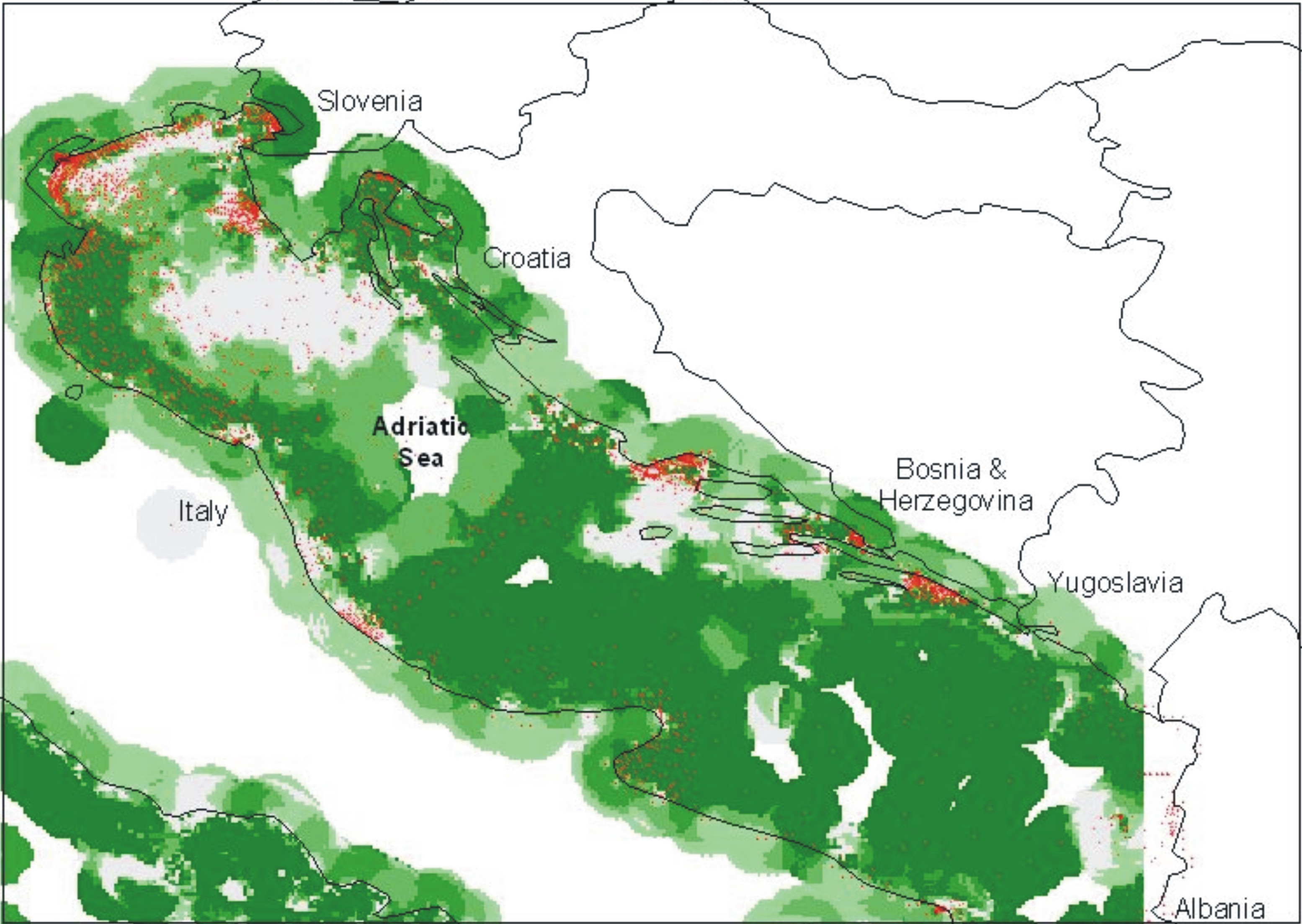
- The IDW interpolation engine is
enhanced. It uses
water depth difference (Z; m) and geographic
distances (X,Y; km) for weighting. With this the 3-dimensionality of
the seafloor is
recognized and results trend more
with depth zones.
- The search radius is varied by
proximity to land (including islands and
reefs), using small radius close inshore, and the maximum for the open
ocean.
- For cells with data the median
is embedded (instead of IDW). This allows areas
surveyed in detail, sharp seabed discontinuities, and the overall
variance to be preserved in
outputs.
- The stock of point data that
feeds each cell's result is subsetted
(usually to 6), evenly prioritizing the nearest data within each
of the 4 quadrants - NSEW. This increases the chance of a result that
reflects the most local data that lies evenly around the gridcell. It
also decreases ill effects from clustering of input data.
- A different search radius is
used for parameters, e.g., rock
exposures are very localized on the seafloor - small radius (~5km);
sand
and mud are very dispersed - wide radius (~20km).
- An uncertainty budget is
computed, involving the spatial
variabilities, measurement errors of the incoming data, disagreement
(variance) between the data within a gridcell, navigational errors.
Statistical
validations
By comparing the
gridded maps including CSI generates, with seafloor properties at sites
that have
not contributed to the grid calculations, we can measure the
performance of the gridding methods.
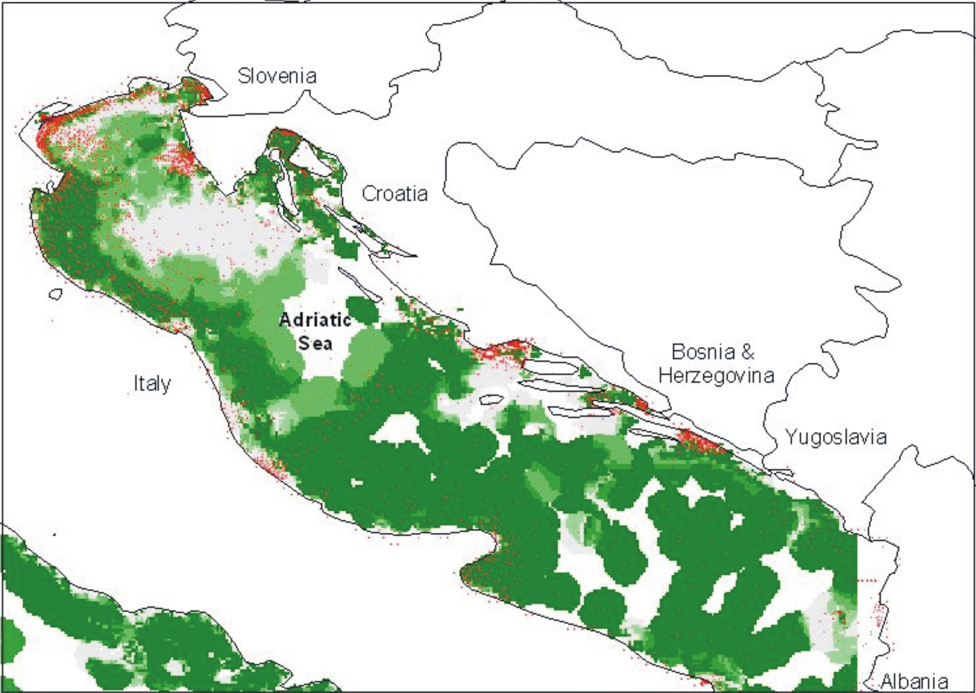
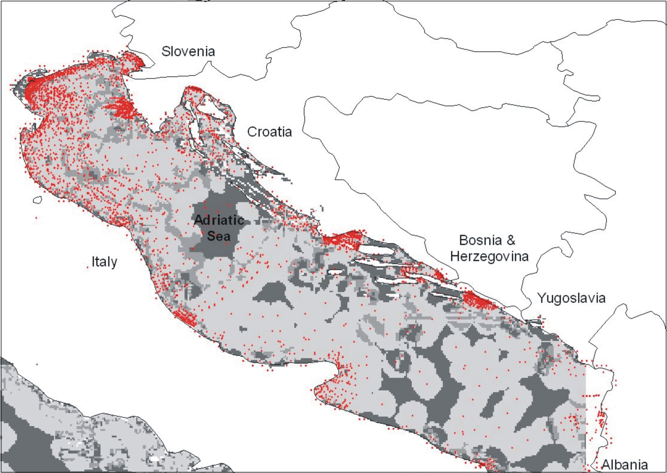
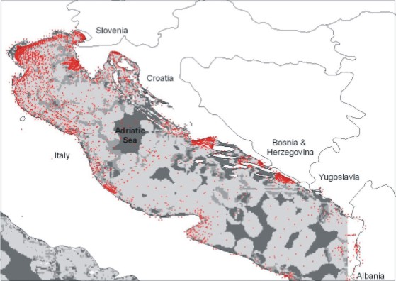
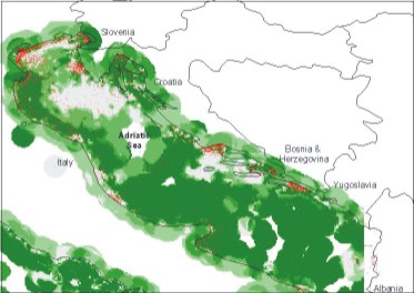
The testbed we used for this covers
the Adriatic Sea (Figs 1-4) and Hawth's Intersect Point
Tool was used to match the point and grid
data.
Consistency test
Consistency of the results in terms of data ranges, means and variance
is tested by comparing the griddings with the actual input data points.
Interpolation
Method |
Av Value
|
SD
Value
|
Mean
Deviation |
| CSI (IDW; variable
search radius up to 20km; XYZ weighting; embedded cell medians;
quadrants) |
50
|
45
|
17
|
IDW (20km search
radius) AV3.x
|
55
|
33
|
17
|
Neighbourhood Mean
(20km search radius) AV3.x
|
54
|
19
|
34
|
Proximity gridding
(Thiessen polygons) AV3.x
|
53
|
44
|
11
|
IDW gridding (6
point; power 2) AV3.x
|
55
|
37
|
13
|
Natural Neighbour
gridding (12 point) AG9.x
|
54
|
37
|
14
|
| Ordinary Kriging
gridding (12 point) AG9.x |
56
|
30
|
25
|
Point
dataset (N=##)
|
54
|
44
|
-
|
Blue:
Good performance; Red:
Poor
Performance.
AV3.x: ArcView version 3.x
AG9.x: ArcGIS version 9.x
Interpolation
skill
The effectiveness of CSI at interpolation between data points was
tested using withheld data (see REF). If this option is selected CSI
lays aside 10% of the points, and computes a grid for testing from the
remainder. Results are given below, compared to performance of other
interpolators working on other datasets (SIC97).
Interpolation
Method |
Av Value (Median)
|
MAE |
RMSE
|
| CSI (As above) |
51
|
26
(Rel: 46%)
|
43
(Rel: 80%)
|
MAE: Mean Absolute Error
(Deviation)
RMSE: Root Mean Square Error (Deviation)
This skill seems low relative to interpolations of the SIC97 and SIC04
benchmarks on radiological and raingauge data. Partly that is because
of the data: spatially very undersampled, diverse marine samplers, low
precision lab analyses, use of parsed word-based data to handle mixed
geologic-biologic substrates, and the 0-100% fixed data range, strong
seabed temporal-spatial variations.
In basic terms the CSI interpolator achieved >20% of results with
zero deviation, 50% within 8% deviation of mud contents.
The calibration suggests that the uncertainties calculated in an error
budget by CSI may be too wide. Nevertheless, frequency
distributions on the grid cell-data deviations (signed and absolute)
and the CSI uncertainty values for cells have similar behaviour (Fig.
10). The uncertainty results may still be correct because they allow
for some uncertainty factors not explicit in the grid deviations.
Technical notes
Choice of IDW
IDW is not markedly less
than the others including Kriging (a Best Linear Unbiased
Estimate) on
scattered environmental data (e.g.,
Cressie 1993; Dubois et al., 1998; Bengio et
al.,
2004). It requires fewer assumptions about
stationarity and continuity/differentiability. IDW is also more widely
comprehended
and
used, and it is somewhat easier to modify in search radius, quadrants,
embeddings, etc.
Artifacts
These are spurious patterns in an interpolation, resulting from the
processing interacting badly with the data distribution. (Figure
numbers.)
- Crescents (4,5): formed when a point passes into a
search
radius, impacting on the result formed by the small number of points
left; wrongly transfers the property of that point to the search radius
rim; in IDW associated with a central "moon".
- Jagged polygons (6): formed in Neighbourood
Statistics
(Thiessen-Voronoi Polygons)
- Double foci (7,8): formed in Natural Neighbour
between close, different valued points.
- Loss of detail (5,9): exceptions are passed over;
depending on settings, this is common from many interpolation engines.
- Paintball (2): In data-sparse areas the search radius
gives out, leaving blank areas.
- Ignore data hull (6,8): The process proceeds without
adapting to the end of data; very pronounced in Proximity and Natural
Neighbour methods
Spatial Indexing
Without an optimized search method, gridding
programs are very slow because of the intense spatial search
requirements. CSI uses a grid-based spatial indexing (Wikipedia 2007)
reading from direct access (DA) files. For cells where data exists a
key is read from the cell-wise DA file 1. That key
points to a record in data-wise DA files 2,3. The key in 2 points to
the first of a chain of data points for the cell, and in file 3 points
to the data for this first point, held in
data-wise DA file 4. On large sets this arrangement gave 10^6
increase of
program speed over brute force, requiring only 2N+1 file reads per cell
with data, and only one for empty cells.
References
- Cressie, N.A., 1993. Statistics for Spatial Data. New
York: Wiley.
- Wikipedia, 2007. Spatial Index. [URL:
"http://en.wikipedia.org/wiki/Spatial_index"]
- Dubois, G., et al. (Eds), 1998.
Spatial Interpolation Comparison 97: Special
Issue. Jl
Geographic Information Decision Analysis, 2(1-2).
- Bengio, S., et al. (Eds), 2004. Spatial Interpolation
Comparison exercise
2004: Special issue. Applied GIS,
1(2), ##.
- Cacchione,
D.A., Grant, W.D. and Tate, G.B., 1984. Rippled scour depressions on
the inner continental shelf off central California, Jl Sediment.
Petrol. 54,
1280–1291.
- Intelmann, S.S., Cochrane, G.R., Edward Bowlby, C.,
Brancato, M.S. and Hyland, J. 2007. Survey report of NOAA Ship
McArthurII cruises AR-04-04, AR-05-05 and AR-06-03: Habitat
classification of side scan sonar imagery in support of deep-sea
coral/sponge explorations at the Olympic Coast National Marine
Sanctuary. Marine Sanctuaries
Conservation Series MSD-07-01. U.S. Department of Commerce,
National Oceanic and Atmospheric Administration, National Marine
Sanctuary Program, Silver Spring, MD. 50 pp. [URL:
"http://sanctuaries.noaa.gov/science/conservation/pdfs/mcarthur1.pdf"]
- Hawth, 2007. Hawth's
Analysis Tools for ArcGIS. [URL:
"http://www.spatialecology.com/htools/"]
- Tomczak, M. 2003. Spatial
Interpolation and its Uncertainty using Automated Anisotropic Inverse Distance Weighing (IDW) -
Cross-validation/Jackknife Approach. In: EUR 2003. Mapping
Radioactivity in the Environment. Spatial Interpolation Comparison
<>1997. EUR 20667 EN, EC. 268 pp. Dubois, G., Malczewski,
G., and De Cort, M. (eds).
Office for Official Publications of the European Communities,
Luxembourg.
|
(Click any image
to enlarge)

1. Input point data distribution
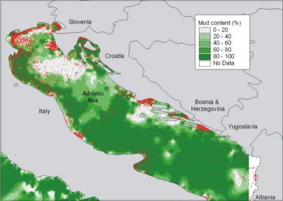
Competent Seabed
Interpolator

2. CSI gridding (IDW, variable search radius, XYZ weighting,
embedded cell medians)
3. Uncertainties for CSI gridding
Download
the CSI software
ArcView 3 (Spatial Analyst)
4. IDW gridding (20km search radius)

5. Neighbourhood Mean gridding (20km search radius)

6. Proximity gridding (Thiessen polygons)
7. IDW gridding (6 point, power 2)
ArcGis 9 (Spatial Analyst)
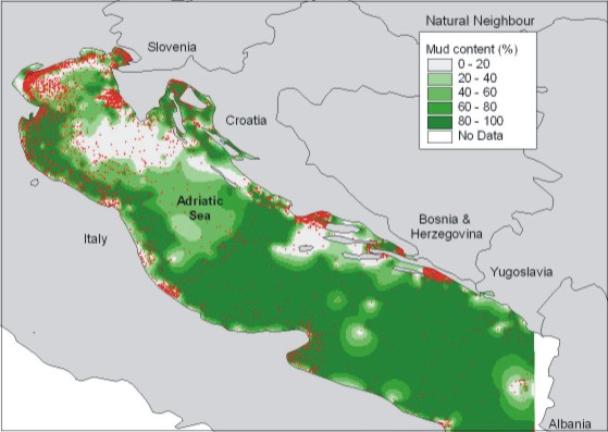
8. Natural Neighbour gridding (12 point)

9. Ordinary Kriging gridding (12 point)
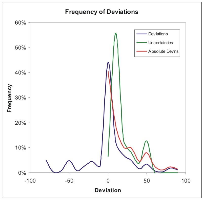
10. Frequencies of grid cell-data deviations,
and of CSI computed uncertainties.
|