The author(s) will give a talk
Mapping ice flow velocity using an interactive, cloud-based feature tracking workflow
1 University of California, Berkeley
2 University of Maryland / NASA Goddard Space Flight Center
3 University of California, Berkeley
4 Stanford University
5 Colorado School of Mines
6 University of California, Berkeley
7 Colorado School of Mines
Observations of ice flow velocity provide a key component for modeling glacier dynamics and mass balance (e.g., Collao-Barrios et al., 2018). Studies also use these measurements as a proxy of glacier change due to climate, ocean, or bed conditions (e.g., Khazendar et al., 2019). While field campaigns may provide precise velocity data for selected glacier sites, deriving velocity from satellite data is usually the only way to obtain velocity for many remote glaciers. The feature tracking technique (also known as pixel tracking, offset tracking, or template matching) is one of the most commonly used methods for deriving ice flow velocity from remote sensing data. This technique computes the cross-correlation between two images of the same glacier acquired at different times and measures glacier motion from offset of the surface features, such as crevasses (e.g., Strozzi et al., 2002).
Despite being cost-effective for mapping ice flow velocity, running a feature tracking workflow is not easy. This is because: (1) Searching for good data can be time-consuming. Users have to define a list of search criteria (e.g., spatial coverage, temporal coverage, maximum cloud cover, orbital tracks) and perform a query on a particular data distribution system. It is usually necessary to change the search criteria multiple times depending on the query results. For data stored on different distribution systems, the learning curve for this step can become even steeper. (2) Fetching and storing the data can be challenging because the source images often come in a large size. For example, a Landsat 8 image pair takes ~1 Gb of disk space, not including the feature tracking results. To calculate the temporal variation of ice flow velocity, one might need 100-1000 Gb of storage for each glacier. (3) There is no standardized routine or workflow for performing feature tracking (e.g., Heid and Kääb, 2012). Multiple cross-correlation kernels, pre- and post-processes, and software packages (e.g., autoRIFT, CARST, ImGRAFT, vmap, and GIV) exist. Still, a detailed intercomparison of recent feature tracking tools has not been conducted. As such, the relative strengths and weaknesses of the different software packages are challenging to evaluate. Selection of a particular workflow and parameter set is often arbitrary and does not guarantee the best results. (4) To date, there have been some online repositories that directly distribute glacier velocity data, such as the NASA ITS_LIVE project (Gardner et al., 2019). While this serves as an essential contribution to many studies, there are still limitations to these readily available datasets. For example, the feature tracking kernel and the workflow are fixed and are applied to certain source data sets. Users can’t use the same workflow on the other datasets or test a different workflow on the same data sets. Besides, the data repository may not be updated with real-time satellite acquisitions. Users have to either wait for new releases or perform feature tracking themselves.
Here we present a Jupyter notebook-based interface that deploys the entire feature tracking workflow from searching the data to visualizing the results. The workflow builds up from these key modular steps: (1) query data, (2) retrieve data and aggregate them to the memory, (3) select feature tracking kernel and parameters, (4) filter data for feature enhancement, (5) perform feature tracking, (6) mask outliers and interpolate results if needed, and (7) visualize and save results. For the first two steps, we develop a library called GeoStacks and use it with the other tools from the Jupyter ecosystem, such as Jupyter-widgets and Geopandas. Steps 3 to 6 are typically included in a feature tracking package, and we implement corresponding algorithms from the CARST software (Cryosphere And Remote Sensing Toolkit; Zheng et al., 2021) in this demo example. CARST will parallelize the image correlation kernel and achieve fast processing time. Each step is fully customizable and extensible, which will help researchers explore new data, compare different algorithms, and validate their results. We use ipyleaflet and Jupyter-widgets and provide an entirely interactive control panel, allowing users to quickly select desired input data and run the feature tracking processes.
In our demo notebook, we query data over Jakobshavn Isbræ, a large outlet glacier of the Greenland Ice Sheet with a history of seasonal flow speed variation (Khazendar et al., 2019; Figure 1). Users can choose to explore the ITS_LIVE velocity dataset or the Landsat 8 imagery and perform feature tracking for the latter. As mentioned above, the feature tracking kernel and all related filters, masks, and interpolation processes are from CARST, but users can easily replace any of them or the entire package with their algorithms or a different feature tracking package (e.g., autoRIFT; Lei et al., 2021). The modules used by this demo notebook, including the GeoStacks and CARST packages, are open-source software and welcome community contributions. The demo notebook represents a way to integrate the entire feature tracking application. Users can also access the same modular content from the tools we use and adopt them in their own projects. Future integration of this work into a numerical glacier model (such as the Open Global Glacier Model, Maussion et al., 2019) or a web-based feature tracking service is also possible.
This work is part of the Jupyter meets the Earth project, supported by the NSF EarthCube program (awards 1928406 & 1928374). The demo notebook is available on Github: https://github.com/whyjz/EZ-FeatureTrack.
Collao-Barrios, G., et al., 2018, Ice flow modelling to constrain the surface mass balance and ice discharge of San Rafael Glacier, Northern Patagonia Icefield. Journal of Glaciology, 64(246), 568–582. doi.org/10.1017/jog.2018.46
Gardner, A. S., et al., 2019, ITS_LIVE Regional Glacier and Ice Sheet Surface Velocities. Data Archived at NSIDC.
Heid, T., & Kääb, A., 2012, Evaluation of existing image matching methods for deriving glacier surface displacements globally from optical satellite imagery. Remote Sensing of Environment, 118, 339–355. doi.org/10.1016/j.rse.2011.11.024
Khazendar, A., et al., 2019, Interruption of two decades of Jakobshavn Isbrae acceleration and thinning as regional ocean cools. Nature Geoscience, 12(4), 277–283. doi.org/10.1038/s41561-019-0329-3
Lei, Y., et al., 2021, Autonomous Repeat Image Feature Tracking (autoRIFT) and Its Application for Tracking Ice Displacement. Remote Sensing, 13(4), 749. doi.org/10.3390/rs13040749
Maussion, F., et al., 2019, The Open Global Glacier Model (OGGM) v1.1. Geoscientific Model Development, 12(3), 909–931. doi.org/10.5194/gmd-12-909-2019
Strozzi, T., et al., 2002, Glacier motion estimation using SAR offset-tracking procedures. IEEE Transactions on Geoscience and Remote Sensing, 40(11), 2384–2391. doi.org/10.1109/TGRS.2002.805079
Zheng, W., et al., 2021, Cryosphere And Remote Sensing Toolkit (CARST) v2.0.0a1. Zenodo. doi.org/10.5281/zenodo.4592619
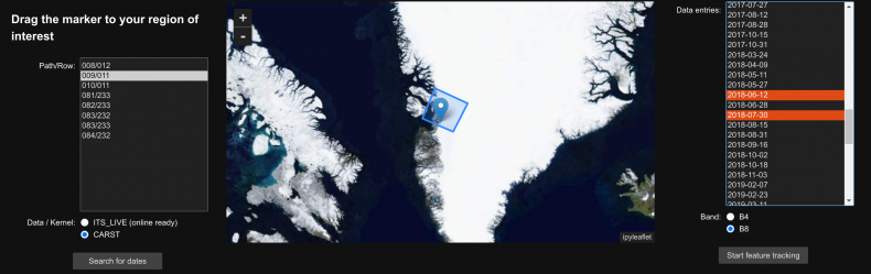
Fig 1.
Jupyter notebook-based graphical interface allows users to explore data, select input and run feature tracking algorithms without much hassle.