Return to db9 Manual
dbSEABED
Input Parameter DefinitionsContents
The handling of date/time information is very difficult. Not only are there many formats with different delimiters and orders of D:M:Y (e.g., US vs International), there is a need to accommodate ranges of dates and uncertainties. There is also the issue of seasons, decades, pre- and post- descriptiors, lost digits in dates, and time zones like 'Local' and 'GMT' / 'UTC'.
Planned Strategy with Dates
Although the parser does not currently work on dates, when implemented,
it will try to follow the certain rules in its outputs. The parser will
be designed to cope with (and translate) as much as possible of the
variety
that people use for dates in the data supplied to us. Notice that each
date will have 2 colon delimiters and will use international DMY order.
The output dates will need a format which allows for uncertainties and incomplete information. dbSEABED prefers a format with a colon as delimiter. For example: "10:Apr:1976" "::1976 to 83" "16 to 20:Apr:1976" ":Apr to May:1976" "16:Apr:19??" ":Apr:>1976" "::<1980" ":Apr:1980".
Symbols '~', '?', '<', '>' and '-' are used to express
uncertainty
and incompleteness in data.
Decade and century ranges may be expressed using "?", such as in "199?"
for 1990's and "18??" for 1800's; also "2?" for 20-something in the
month.
Months will be 3-letter abbreviations:
Jan,Feb,Mar,Apr,May,Jun,Jul,Aug,Sep,Oct,Nov,Dec.
Seasons may also be allowed Sum,Win,Aut,Spr.
The US/International format problem
In data being entered to dbSEABED if a US date is submitted with the
month as a numeric, it can be entered with a 'US' somewhere in the
string,
such as in : "[US]06121984". dbSEABED will output this as "12:06:1984"
in international system.
Whether the dates in a survey are International or US, and whether Local or Zulu time, can also be specified for a whole dataset (or section of dataset) at a time using the dedicated fields in the SVY theme lines.
Planned Strategy for Time
Output times will have this format: HOUR:MINUTE:SECOND:ZONE. Where
they are necessary, symbols expressing uncertainty (see above) will be
included, including for TimeZone.
dbSEABED works in the WGS 84 spheroid system using decimal latitude
and longitude.
Data sets which have been reported or published in other systems need
to be converted before incorporation into the database.
WGS84 positions lie within 1m of positions in the new GDA 2000 (GPS
based) system.
Latitudes and longitudes are held to precisions of approximately 1m,
which is usually 5 decimal places.
Of course, many datasets will have their sample locations reported
to much less accuracy, usually >300m.
Most water depths in dbSEABED are not tidally corrected and many echosounder depths may not be corrected for local variations of sound speed.
Subbottom depths (including 'Top' and 'Bot') are expressed in metres to a precision of 1cm (2 decimal places) in dbSEABED.
Grainsizes appear to obey a logarithmic distribution of abundances
in
samples, so they are usually reported on a log base 2 scale.
This is related to D, the mm grainsize of the particles, by:
Median grainsize is the phi size where half the sample is finer and half is coarser.
Average, or mean, grainsize is the first statistical moment of the grainsize distribution over a number, n, of classes:
The phi grainsize which is the most abundant in the sample:
Modes and their peak abundances are represented in a coded way in
inputs
as follows:
3.3[15] ;4.5 [13] ;8 [10] where the number inside the brackets is the
% frequency of the peak class specified by
the phi value ahead of the brackets. Where no % frequency value is
available for a mode, it can be entered like "3.4[] ;5.6 [ ]".
The semi-colons are optional, the brackets are mandatory; spaces are allowed between brackets and values.
Percentiles and quartiles are read directly
from
the cumulative grainsize distribution of a sample:
The larger percentile / quartile is the
coarsest:
P84 coarser than P16; Q3 coarser than Q1.
P50 and Q2 equate to the median grainsize.
Unfortunately, the terms 'mean', 'sorting',
'skewness'
and 'kurtosis' have been abused over the years, applied to a range of
very
different functions.
The earliest usage appears to be in Krumbein
& Pettijohn (1938) who employed graphical measures. Other graphical
definitions have been by Inman (1952) and Folk (1974).
Once electronic computing became widely
available,
these graphical measures were gradually superceded by the more rigorous
statistical measures of dispersion.
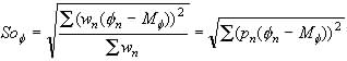
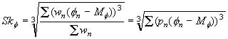
In dbSEABED the terms relate to the statistical (moment) measures.
They
are in fact, the first to fourth statistical
moments
of the grainsize distribution of a sample over a number, n, of
classes
of central phi size, ##.
|
|
Standard Deviation | |
 |
||
|
|
|
|
 |
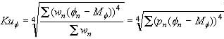 |
The class frequencies are usually in terms of weight (wn), but if fractional (pn) the second form of relation applies.
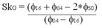
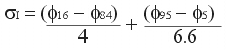
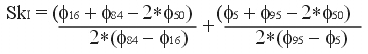
Inman (1952) proposed a series of graphical
measures
of central grainsize, sorting, symmetry and peakedness that have been
widely
used since. They use percentile phi values, P5, P16, P50, P84 and P95.
|
|
(Inman) Graphic Standard Deviation | (Inman) Graphic Skewness |
|
|
|
 |
Folk (1974) introduced an extra set, to recognize the effects of
outlying
parts of the grainsize distributions on these statistics.
| (Folk) Inclusive Graphic Standard Deviation |
|
 |
 |
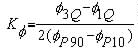
These measures of central grainsize, sorting,
symmetry and peakedness by Krumbein & Pettijohn (1938) use
quartiles
in the grainsize distributions of samples. In the following equations,
Q represents 25%.
|
|
(Quartile) Standard Deviation | (Quartile) Skewness |
|
|
|
|
|
 |
D90 and D10 are the mm values of grainsize at the 10 and 90 percentiles (their notation should be DP90, DP10, D denoting mm grain diameter). Similarly there are median and quartile mm grainsize statistics: 'D50' (=Q2), 'Q1', 'Q3' (properly DP50, DQ1, DQ3).
The Coefficient of Uniformity is defined as the ratio D90 / D10.
PettiJohn (19##) tabled some statistics based
on mm grainsize:
| Coefficient of Sorting | Coefficient of Skewness |
|
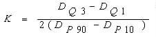 |
Currently, of these only the Coefficient of Sorting is called for in dbSEABED.
Munsell Codes provide a description of percieved colour in terms of Hue (Colour), Value (Luminance) and Chroma (Intensity). In 7.5GY 6/4 '7.5GY' is the Hue, 6 is the Value and 4 is the Chroma. Sediment and rock colours are usually described by comparisons with the Geological Society of America 'Rock Colour Chart'.
Hue is defined as steps of 2.5 inside 10
sectors
of a colour wheel (see below), the sectors passing from red through
yellow,
green, blue and purple, back to red (R, YR, Y, YG, G, BG, B, BP, P,
PR).
Pure whites and blacks are denoted from 5N 1/0 through to 5N 9/0
respectively.
The Munsell scheme does not provide an undistorted psychrometric colour
space. But it is by far the most widely used colour measurement system
in earth sciences.
 The Munsell colour wheel with Hue in circumference, Chroma in radius and Value in Axis. (From Gretagmacbeth) |
Munsell Codes in dbSEABED must be complete in
order for successful data mining.
Back to top
Following work mainly based on SPI camera surveys, the depth of the top of the reduced layer is defined as the depth of change from oxic colours brown/orange/red to black/dark grey/green. The change to reducing conditions may also be accompanied by increases in sulphide gas and pyrite. The change is also the depth down to which sediments are oxidized.
For the SPI methods, an area-averaged depth is reported, the Redox Potential Discontinuity (RPD; Iocco and others 2000).
![]()
Chris Jenkins (Email)
INSTAAR, University of Colorado
13-Aug-2004