dbSEABED
Dealing with Polygon /
Polyline
Data
This page is superceded by New Polygon Page
|
Contents
Return to db9 Manual
General
dbSEABED seeks to preserve the spatial resolution of the original
input
data, especially where that data is point sampling data. But polygons
(also
polylines and grids, henceforth all in term "poly coverages") are
summaries
of sampling data with decreased spatial resolution.
Polygon data is also difficult because, if it was to be accepted
wholly
as areas: (i) it would cover over point samplings in its area, (ii) it
cannot contribute to interpolations of point data, and (iii)
overlapping
polygons of different class (eg, "sand' and "bryozoal sand", perhaps
from
separate studies) cannot be reconciled on one map.
To solve these problems, dbSEABED transforms poly coverages to point
representations, area griddings, or outline nodes by generating points
which have the spatial distribution of the polygons/grids/polylines and
their geological attributes. There are a number of choices available to
the user:
(i) render the outside perimeter or the inside area of the object
(ii) use rectilinear or random point gridding,
(iii) with or without a blank buffer just inside the perimeter.
The conversion to points is performed at approximately the same scale
as the spacings between the nodes that define the polygon/polyline or
the
cells of a gridding.
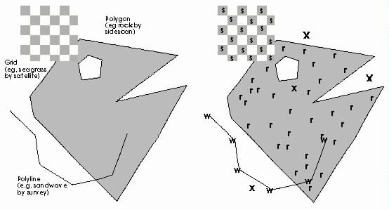
An illustration of the methods is shown below. Once points are
created
from the polygon, polyline and grid, that data can be interpolated with
actual sampling data to produce an integrated map. Notice the
complication
of salients and islands on the polygon; these are fully dealt with in
the
dbSEABED software.
 Interspersing polygon, polyline and grid topologies with
point
data types in dbSEABED.
Interspersing polygon, polyline and grid topologies with
point
data types in dbSEABED.
a. Poly coverage elements; b. Conversion to points and combination
with other point samplings.
Letters represented the generated points: r – points for rock area
polygon; s – points for seagrass gridding;
w – points representing sandwave crest. X – represent nearby actual
sampling sites.
|
Back to Top
Preparing the Mid/Mif files
dbSEABED uses the ASCII MapINFO(R) Mid/Mif format to store original
information on polygons, polylines and grids. The format is easily
readable
and understood, it is widely used and can be easily generated from many
GIS including MapINFO(R) and ArcVIEW(R).
- If the user has a file of polygons in (say) ArcVIEW(R) shape
files
(*.shp/*.shx/*.dbf)
or ArcINFO export format (*.e00) then the ArcAVENUE(R) script
"shp2mif.ave"
is available within ArcVIEW(R) to generate the Mid/Mif file pairs.
- If the user has MapINFO(R) *.tab/*.dat/*.map poly coverage then
in
MapINFO(R)
use <Table/Export/MapInfo Interchange format> to convert.
The files for processing are pointed to in the file "us8_MIF.asc" for
west
coast USA and "au8_MIF.asc" for Australian waters. A typical entry
consists
of a normal "SRC" line describing the metadata for the poly coverage,
followed
by a "MIF" line providing details of the poly coverage pointed to and
the
rendering that is to be applied.
The Mid/Mif data files are placed in the subfolder "_Data\_MifData".
It is important that they be PC format rather than MAC or UNIX: it
affects
the line lengths. To transform, import them into MapINFO(R)
(<Table/Import/MapInfo
Interchange format>), open the resulting table
(<File/OpenTable>), then
save it over the original Mid/Mif by a re-export (see above).
While some coverages have individually attributed objects, many are
of just one seabed type.
- If the former is the case, the attributes are carried in the
"*.Mid"
file.
The user nominates which column in that file is to carry the
attrributions
by the syntax "Column# n" (eg, "Column# 2") in the attributes field of
the MIF line in "_Data\au8_MIF.asc".
- If not, then dbSEABED allows the user to override any attributes
and
assign
the attribute at rendering stage, for example "rck" or "klp". The
description
is entered in the attributes field of the MIF line in
"_Data\au8_MIF.asc".
Back to Top
Running the rendering program
The program "db8_render_poly.bas" is run from its shortcut in the
Host
Folder. It works through all MidMif files pointed to in the data file
"us8_POLY.asc"
(or "au8_POLY.asc") which is held in the "_Data" subfolder (document
version
held in "_Data\_Documents") and which in structure is like a normal
dbSEABED
ASCII Data Resource File.
No latitude/longitude limits are applied at this stage.
Back to Top
Combining with point data
The outputs from "db8_render_polys" are placed automatically in the
folder "_Data" where they are available for processing by the main
dbSEABED
program "db8_process". From there the points generated from the poly
coverages
are represented in the EXT/PRS/CLC and FAC/CMP files alongside actual
sampling
points. The generated points are named for the poly coverage file they
originated from, for example "coffs_rck.mif".
Latitude/Longitude and Water Depth limits can be placed on the
points
at this stage using the usual facility for all points in
"UserFile.txt".
Using the EXT/PRS/CLC and FAC/CMP files, the points may be graphed,
mapped and interpolated in the same way as directly sampled points.
Back to Top
Return to db9 Manual

Chris Jenkins (Email)
INSTAAR, University of Colorado
5-Feb-2002